How to Make Line Chart Data in Excel: Layout Rules That Stick

Learn how to make line chart data in Excel: date columns, series headers, tables, and fixes for broken axes.
Most “how to make line chart data in excel” frustration happens before Insert → Chart. The chart wizard runs fine; the table is sideways, dates are text, or a Total row sits inside the selection. This guide defines the matrix layout line charts expect, how to format dates, when to use Excel Tables, and how to fix axes after import from CSV or Google Sheets.
For chart insertion steps after the grid is clean, read How to Make a Line Chart in Excel. For download and template options, see the pillar Download Google Spreadsheet Line Chart Template: Choose and Use. More guides: template guides and tips.
Key takeaway: Line chart data is a matrix: ordered labels in column A, numeric series in columns B onward, one header row, no internal blanks, no totals in the plot range.
The matrix layout line charts expect
Excel Easy and Microsoft Support show the same picture:
| Period | Series A | Series B |
|----------|----------|----------|
| Jan 2026 | 100 | 80 |
| Feb 2026 | 120 | 85 |
Row 1 = headers (become legend entries). Column A = categories — ideally Excel serial dates. Columns B+ = numbers only.
[TABLE: Layout rules]
| Rule | Reason |
|---|---|
| One row per period | Each point needs one x-value |
| Short series headers | Legend readability |
| No merged cells in data | Breaks range expansion |
| Sort oldest → newest | Line reads naturally left-to-right |
| Keep notes outside range | Text in value columns breaks plotting |
Warning: Tidy “long” data (Year, Month, Metric, Value) is great for pivots but wrong shape for direct charting — summarize to wide matrix first.
Dates: the axis that breaks most imports
CSV exports and Google Sheets copies often land as text that looks like dates. Symptoms: every point evenly spaced but wrong order, or a flat line at zero.
Fix sequence:
Fix date column
- Select column A → Data → Text to Columns if needed, or use
DATEVALUEin a helper column. - Apply a date number format (yyyy-mm-dd or locale equivalent).
- Click chart → Format horizontal axis → Axis Type → Date axis.
- Confirm gaps match real elapsed time (weekly vs daily).
DataCamp notes beginners often skip step 3 — do not.
Use Excel Tables when data grows weekly
Convert the block to a Table (Ctrl+T). Name it KPI_Data. Benefits:
- Structured references in formulas (
[@Sales]). - Auto-expand when you paste new rows at the bottom.
- Charts tied to the table can grow with new periods.
When you add a column for a target line, extend the table width before editing chart ranges — see Add Target Line to Excel Chart.
Product highlight: A table-backed chart reduces “why is last week missing?” tickets because the blue data range expands with the table.
Multiple series without wide-table chaos
Each metric gets its own column — not its own row. Three KPIs over twelve weeks = column A plus three value columns, not thirty-six rows of long format unless you pivot first.
If you must combine sheets, use Select Data → pick ranges on other tabs, or define dynamic named ranges with OFFSET/INDEX — advanced; most teams should keep one source tab.
For visual limits with many columns, read Multiple Line Chart Excel.
Totals, blanks, and zeros
- Totals — compute below the table or on a dashboard tab; exclude from chart selection.
- Blanks — Excel draws gaps; decide if gaps mean “no data” or “zero” and fill accordingly.
- Zeros — legitimate zeros plot at the axis; do not delete unless the metric truly did not exist.
Template as a layout reference
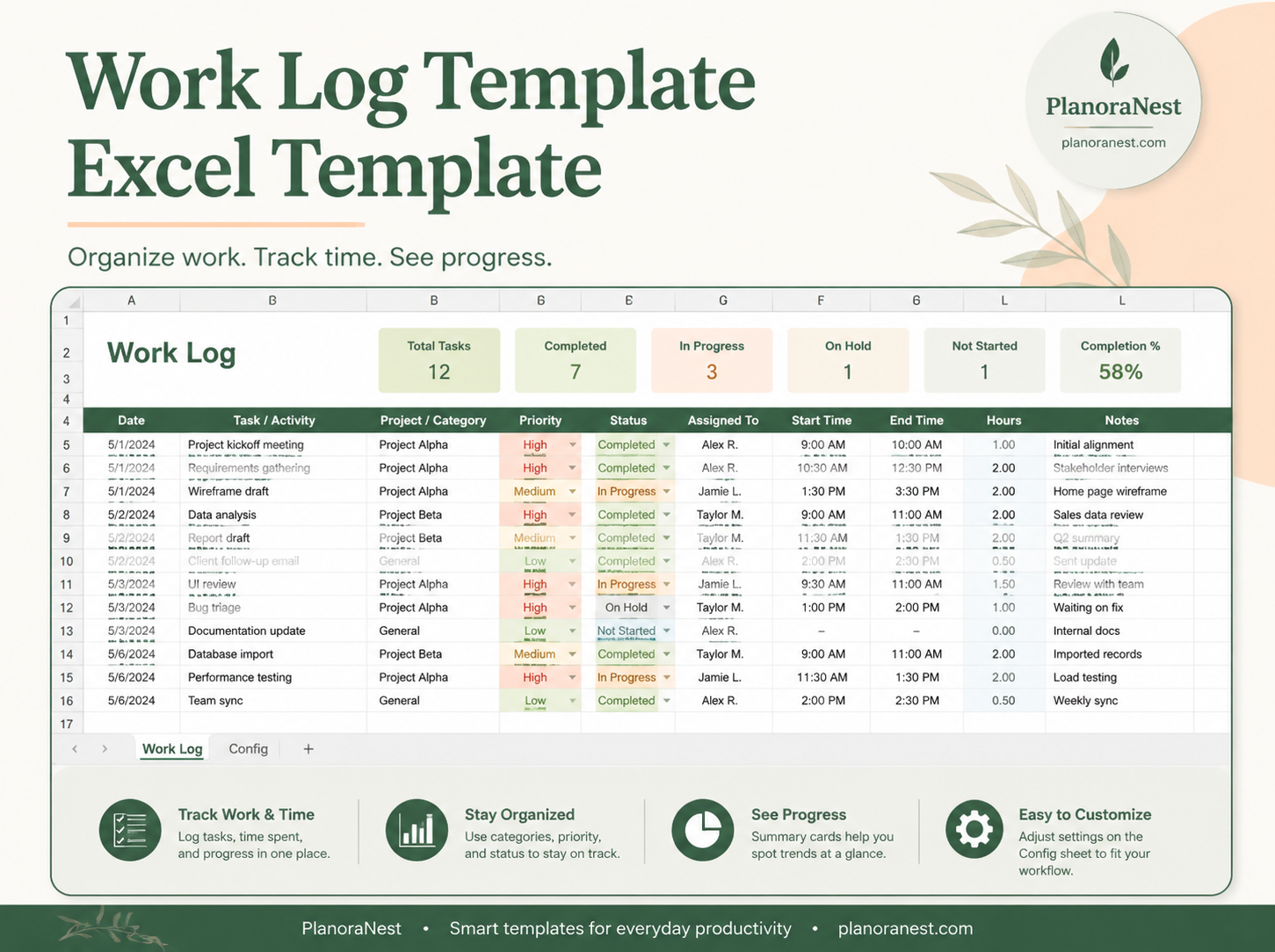
The PlanoNest line chart template ships example tables — temperatures, daylight, sales, milestones — showing date columns and target-line helper columns. Use it as a layout reference even if you replace sample numbers entirely. One-time purchase, instant download; product page has pricing. Collection: KPI Dashboards.
Import from Google Sheets or CSV
Google Sheets exports often produce text dates — rerun date conversion in Excel. CSV may drop leading zeros in week labels — prefer ISO dates in the source system. After import, open Excel Line Chart if you need formatting guidance post-data-prep.
Pivot long data to a wide matrix
Exports from BI tools often arrive tall: Date | Metric | Value. Line charts want wide: Date | MetricA | MetricB. Use a PivotTable: rows = Date, columns = Metric, values = Sum of Value. Copy the pivot output as values to a chart tab so refreshing the pivot does not fight chart ranges. Clear blank pivot cells before charting — pivots love to insert empty columns that become phantom series.
Named ranges for growing tables
Define a dynamic name with OFFSET/INDEX or use structured table references like KPI_Data[Sales]. Point the chart series at the name instead of $B$2:$B$50. When the table grows, the name expands — fewer broken charts after month-end close. Document the name on Start Here so the next editor knows which range feeds which series.
Frequently Asked Questions
How should data be arranged for a line chart in Excel?
Dates in column A, metrics in columns B+, headers in row 1, no blanks or totals inside the range.
Why are my dates not spacing correctly?
Text dates or category axis — convert to real dates and choose Date axis.
Should I use an Excel Table?
Yes when you append periods regularly.
Can I chart data from multiple sheets?
Yes via Select Data or named ranges.
Where do totals belong?
Outside the chart selection.